Statistics for Thickness Data: Predicting What You Didn't Measure
How statistics improves inspection decisions: extreme value analysis for the deepest pit you didn't measure, and how many CMLs a reliable average needs.
By Syed Hasan17 Nov 20265 min read
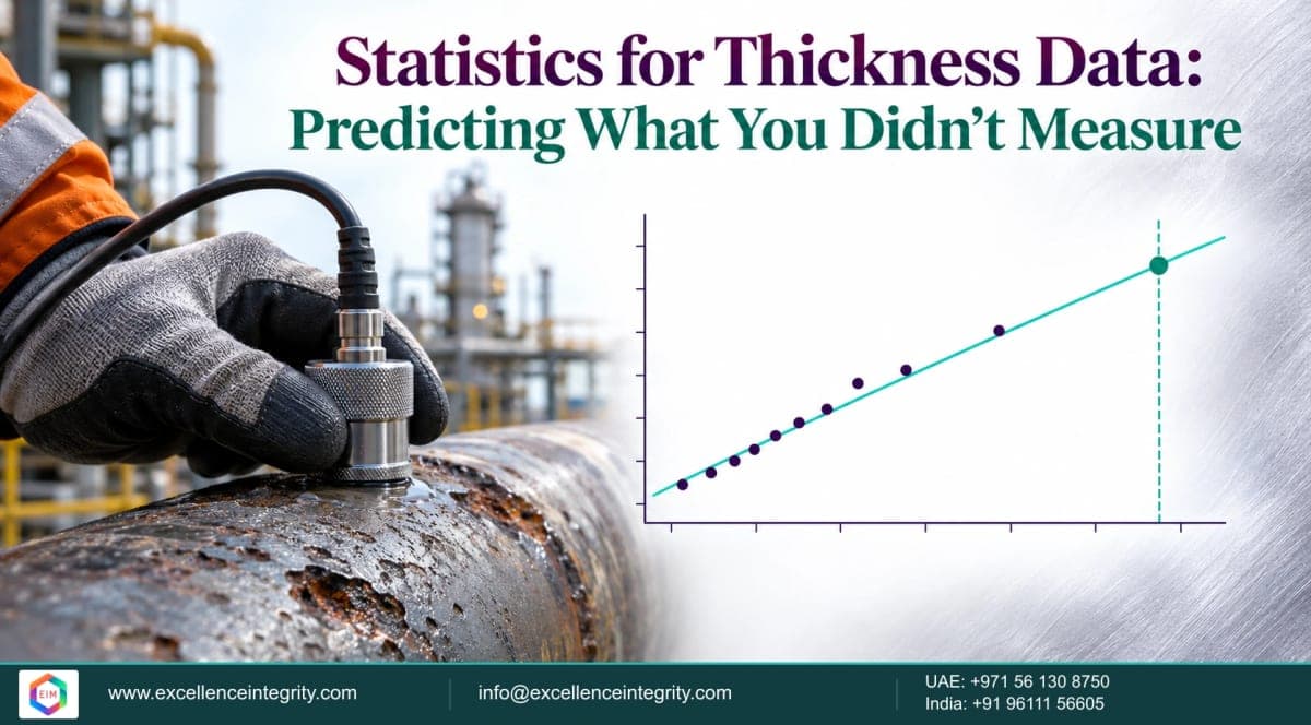
Inspection is sampling. A tank floor scan covers part of the floor; a piping circuit has a few dozen CMLs out of thousands of square metres of wall; a corrosion coupon sees one spot. Every decision drawn from those samples carries uncertainty, and two statistical tools answer the questions inspectors care about most: how deep is the worst pit I didn't measure, and how many readings do I need to trust an average rate?
Short answer: Extreme value analysis fits a Gumbel distribution to the maximum pit depths from several sample areas and extrapolates to the whole surface, predicting a deepest pit that is usually deeper than anything measured. For general corrosion, the confidence in a circuit's average rate improves with the square root of the number of CMLs: going from 3 to 10 CMLs helps a lot; going from 20 to 40 helps much less.
Part 1: the deepest pit you didn't measure
Suppose you inspect ten sample areas on a tank floor, each covering 1% of the floor, and record the deepest pit in each. The deepest you found is 2.2 mm. Is that the deepest pit on the floor? Almost certainly not: you have looked at only 10% of it. The maxima of samples follow a known statistical shape, the Gumbel or extreme value type I distribution, which lets you estimate the maximum over the whole area.
The method
- Take the maximum pit depth from each of n equal sample areas.
- Fit a Gumbel distribution. A simple method uses the sample mean and standard deviation: scale β = s × √6 / π, and location μ = mean − 0.5772 × β.
- Set the return period T = total area / area of one sample.
- Predict the maximum: depth = μ + β × y, where y = −ln(−ln(1 − 1/T)).
Worked example
| Step | Value |
|---|---|
| Ten sample maxima (mm) | 1.0, 1.1, 1.2, 1.3, 1.4, 1.5, 1.6, 1.8, 1.9, 2.2 |
| Mean and standard deviation | 1.50 mm and 0.38 mm |
| β = 0.38 × √6 / π | 0.296 mm |
| μ = 1.50 − 0.5772 × 0.296 | 1.329 mm |
| Return period T (each sample is 1% of the floor) | 100 |
| y = −ln(−ln(1 − 1/100)) | 4.60 |
| Predicted deepest pit = 1.329 + 0.296 × 4.60 | 2.69 mm |
The predicted deepest pit, about 2.7 mm, is half a millimetre deeper than anything measured. On a 6 mm floor, that is the difference between 3.8 mm and 3.3 mm remaining, which can change an inspection interval. Extreme value statistics for pitting are recognised in ASTM G46, and are widely used for tank floors and piping.
Cautions
- Samples must be comparable: equal areas, same damage mechanism, same inspection method.
- One mechanism at a time: mixing, say, product-side pitting near the sump with general floor pitting distorts the fit.
- Check the fit: points should lie close to a straight line on the Gumbel plot.
- Extrapolate with care: the further the return period beyond the data, the wider the uncertainty.
Part 2: how many CMLs do you need?
For general corrosion, the question is different: how well do you know the circuit's average rate? If the rate varies from CML to CML with a standard deviation s, the 95% confidence half-width of the average from n CMLs is about t × s / √n, where t comes from Student's t-distribution.
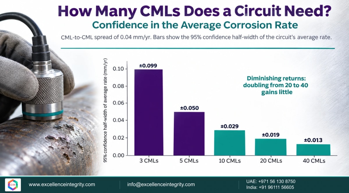
With a CML-to-CML spread of 0.04 mm/yr, three CMLs leave the average uncertain by about ±0.10 mm/yr, as large as many actual rates. Ten CMLs narrow it to about ±0.03 mm/yr. Twenty give ±0.02, and forty ±0.013: a small gain for twice the work. That is the statistical case behind CML optimisation: enough readings to know the average, then effort moved to the locations where localised damage hides.
This assumes general, fairly uniform corrosion. Where damage is localised, more spot CMLs are not the answer; scanning and extreme value methods are. And measurement error adds its own uncertainty, covered in UT thickness errors.
Putting it to work
- Plot your data before trusting any average: histograms and probability plots show outliers and mixed populations.
- Separate mechanisms and locations into comparable groups.
- Use extreme value analysis where localised damage and partial coverage meet, such as tank floors and pitted piping.
- Report uncertainty, not just a single number, when a decision depends on it.
- Re-check after each inspection as more data arrives.
Learn more with EIM
EIM's self-paced Digital Asset Integrity & Predictive Analytics programme covers turning inspection and condition data into decisions, and spotting early when the data cannot support the claim. It is built for inspection and integrity engineers moving into data-driven roles and reliability engineers building predictive programmes. See the programme. For operators, EIM's asset integrity services include CML rationalisation and corrosion review. EIM is an independent training provider.
Frequently asked questions
What is extreme value analysis in corrosion?
A statistical method that fits a Gumbel distribution to the maximum pit depths from sample areas and extrapolates to predict the deepest pit over a larger, uninspected area.
What is the return period?
The ratio of the total area of interest to the area of one sample. It sets how far the Gumbel fit is extrapolated.
Why is the predicted maximum deeper than the measured one?
Because only part of the surface was inspected. The deepest pits on the whole surface are statistically likely to be deeper than those in the sampled areas.
How many CMLs does a circuit need?
Enough to estimate the average rate with useful precision, which depends on how much rates vary between CMLs. Precision improves with the square root of the number of CMLs, so the first few additional CMLs matter most.
Do the codes allow statistical analysis?
Yes. API 510 and API 570 allow statistical analysis of thickness data, and ASTM G46 recognises extreme value statistics for evaluating pitting.
Sources
- ASTM G46, Standard Guide for Examination and Evaluation of Pitting Corrosion (statistical methods). Cited, not quoted.
- Gumbel extreme value distribution: standard statistical references.
- Worked examples prepared by EIM. Checked 7 October 2026.
Free mock tests
Preparing for an API, AMPP (NACE), CSWIP or CMRP exam?
Choose your certification and try a free mock test.
SMRP